Model Accuracy Assessment

We assess accuracy of GNN models in a number of ways, at both the local and regional scales. In general, GNN vegetation maps are appropriate for landscape to regional-scale analyses but are insufficiently accurate for local or stand-level applications.

The following examples are from the 2006 GNN model covering Western Washington for the Northwest Forest Plan project.

Local Scale Accuracy

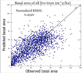
Observed vs. Predicted Plot Attributes

We create scatterplots to compare the observed plot values against predicted (modeled) values for each plot used in the GNN model. The observed value comes directly from the plot data, whereas the predicted value comes from the GNN prediction for the plot location.

We use a modified leave-one-out cross-validation approach, based on a pixel's second nearest-neighbor. We develop our models with all plots, but in determining accuracy, we don't allow a plot to assign itself as a neighbor at the plot location. This approach yields similar accuracy assessment results as a true cross-validation approach, but probably slightly underestimates the true accuracy of the distributed (first-nearest-neighbor) map.

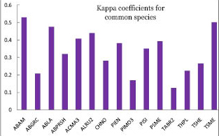
Species Kappa Coefficients

One accuracy measure we use for the species distribution variables is based on Cohen's kappa coefficient, which is a statistical measure of reliability that accounts for agreement occurring by chance.

The equation for kappa is:

kappa = (Pr(a) - Pr(e))/(1.0 - Pr(e))

where Pr(a) is the relative observed agreement among raters, and Pr(e) is the probability that agreement is due to chance.

Vegetation Class Error Matrix

We create an error matrix for vegetation class assignments at plot locations. Cell values are model plot counts. Dark gray cells represent plots where the observed class matches the predicted class and are included in the percent correct. Light gray cells represent cases where the observed and predicted differ slightly (within +/- one class) based on canopy cover, hardwood proportion or average stand diameter, and are included in the percent "fuzzy" correct.

Observed Class	Predicted Class
Observed Class	Sparse	Open	Blf- Sm	Blf- Md/Lg	Mix- Sm	Mix- Md	Mix- Lg	Con- Sm	Con- Md	Con- Lg	Con- VLg	Total	% Correct	% FCorrect
Sparse	12	33	2	0	4	1	0	5	3	0	0	60	20.0	75.0
Open	111	49	2	0	9	5	0	39	6	1	0	122	40.2	90.2
Blf - Sm	1	4	4	6	8	5	0	4	0	0	0	32	12.5	68.8
Blf - Md/Lg	0	1	5	9	3	19	1	2	4	0	0	44	20.5	77.3
Mix - Sm	0	3	1	5	19	13	0	16	7	0	0	64	29.7	81.3
Mix - Md	0	1	2	6	17	28	2	7	23	4	0	90	31.3	84.4
Mix - Lg	0	0	0	1	0	5	3	0	3	1	0	13	23.1	76.9
Con - Sm	1	16	0	0	29	14	0	215	144	16	0	435	49.4	92.9
Con - Md	0	6	0	0	7	25	1	69	410	119	13	650	63.1	95.8
Con - Lg	0	0	0	0	0	4	1	7	130	148	48	338	43.8	96.7
Con - VLg	0	0	1	0	0	0	0	1	22	91	33	148	22.3	83.8
Total	25	113	17	27	96	119	8	365	752	380	94	1996
% Correct	48.0	43.4	23.5	33.3	19.8	23.5	37.5	58.9	54.5	38.9	35.1		46.6
% FCorrect	92.0	92.9	70.6	81.5	85.4	75.6	87.5	92.9	94.0	94.5	86.2			91.5

Regional Scale Accuracy

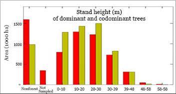
Area Distributions from Regional Inventory Plots vs. GNN

We create histograms to compare the distributions of land area in different vegetation conditions as estimated from a regional, sample- (plot-) based inventory (FIA Annual plots) to model predictions from GNN (based on counts of 30m pixels).

The stand height histogram to the left is just one example of an area histogram included in GNN accuracy assessment reports. The reports contain histograms for a variety of plot variables including tree basal area, canopy cover, quadratic mean diameter, snag volume, etc.